
This page provides .WAV files that can be combined with audio tracks to perform your own evaluation of the audibility of noise, both the unavoidable white noise and the excess noise (mostly low frequency) that is present in differing amounts based on the resistor technology.
This is one of three posts related to resistor noise. The other two related ones are:
- Resistor noise presentation from the Boston AES 27-Feb-2018 meeting
- Resistor noise paper
During the presentation some examples of using various sound clips combined with simulated resistor noise were presented. The simulated resistor noise includes Johnson-Nyquist noise (i.e. white noise due to the thermal noise, a function of resistance and temperature) and 1/f noise (i.e. a pink noise spectrum, also called flicker noise, and only a function of current and resistor construction). For a resistor the 1/f noise component can be defined by a dimensionless number called the Noise Index, and provided in dB. For parts with high frequency noise that is the same as the theoretical Johnson noise value (which is just about all resistors; carbon composition being the ones that glaringly fail in this category), the NI provides a simple figure of merit. For a quick overview of NI see this article (though apparently written to sell their most expensive parts).
These files were created in Audacity by mixing pink and white noise at different levels. This is more or less the same as controlling the Fc (knee) in the noise spectrum. It can also be thought of changing the noise index, but an actual noise index is a representation of the noise voltage measured across a decade with a DC voltage applied. Adding gain or using the signals in a digital representation referenced to 0 dBFS ( dB Full Scale) removes the meaning of the NI. If one applies the same gain to different noise spectrums it is still valid to compare the results of parts with two different NIs.
The actual noise generated by a resistor is a function of NI and the applied voltage. The noise that makes it to the output of the circuit using a resistor is a function of the circuit topology. A resistor in the signal path will have a direct effect on the output signal than a resistor used as part of a bias divider with a large filter capacitor; the latter will have no effect as the capacitor will filter the noise in the audio band.
Listening test
This listening test can therefor not tell you what NI is good or bad. That can only be determined by analyzing the part and the circuit. What it can tell you is what level of noise at the output would be objectionable (or perhaps we should use the word audible) to the listener. This too is a function of where the signal is listened to; the background noise in a typical home, a custom home theater, recording studio, a car, and headphones are all very different and will mask the signal (the signal being the noise) differently based on psychacoustic frequency sensitivity and masking effects.
In the demonstrations used during the paper presentation the mixing of noise with clips from 2L is performed. 2L has graciously provided segments of very high quality audio in a variety of high resolution formats to the audio community.
You should also use clips of your own favorite performances as part of the evaluation. To avoid long processing times you should extract sections of interest from the overall piece, no more than a minute or two of content as you will want to replay them many times with differing noise levels.
You should verify that the selected content has peaks close to 0 dBFS. Check the RMS signal level of typical periods of the content to make sure it’s not, on average, exceptionally loud (compressed) or soft, as either of those would make a typical listener adjust the volume control on that track to compensate, which would raise or lower the noise in absolute terms relative to 0 dBFS. In Audacity the plug-in ACX check works well for this, though that is not its purpose. It’s also worthwhile to run the clip-check as you really don’t want to use content like that – for anything.
In the this experiment this is a Just Noticeable Difference (JND) type test as it removes the need for performing double blind tests on yourself. Listen to the clips and adjust the volume to be at a comfortable level for extended listening. Once started do not change the volume. Controlled experiments would of course be performed with minimal background noise, and measured SPL to ensure the system levels are traceable. That level of rigor is not needed if we’re willing to accept that we could be off +/- 6 dB or more, which sounds like a lot but generally even under the most optimistic audibility assumptions it can still serve as guide to inform design choices.
Here’s an example created with this procedure of the 2L clip Joseph Haydn: String Quartet In D, Op. 76, No. 5 – Finale – Presto combined with pink + white noise with Fc=800 Hz and at a level of – 50 dBFS RMS.
With a RMS signal level around -22 dBFS RMS the noise is only 30 dB lower and therefor easily audible in this illustrative example.
The sample noise files
There are two types of files, one with the Fc at 100 Hz and the other with an Fc of 800 Hz. Most of the high quality resistors are going to have a NI that corresponds to the Fc 100Hz. Really noise parts, like thick film resistors, will be much noisier than the Fc 800 Hz example.
For convenience three copies with different RMS levels have been provided as Audacity allows easy +/- 30 dB gain adjustment on tracks. The -60 dBFS RMS one is therefor the most useful for experiments with audibility.
Fc 100 HZ: -10 dBFS RMS -60 dBFS RMS -80 dBFS RMS
Fc 800 Hz: -10 dBFS RMS -60 dBFS RMS -80 dBFS RMS
The noise files are provided as .wav files as they can not be losslessly compressed and lossy compression will change them in unpredictable ways. They are 16 bit with 44.1 kHz (mono) files as those are more than sufficient sample rate and bit depth for these experiments. (one might argue for the -80 dBFS RMS file that a 24 bit format might be more appropriate). If the files being only 16 bits is a concern then use the -10 dBFS RMS file and change its level after converting to 24 bits.
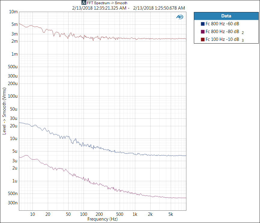
Some of the noise files were played back from a PC/soundcard in to an AP515 in the same manner used in the paper to measure the resistor NI. The plot below illustrates the typical results.
How to use these files with Audacity
It is suggested that you set Audacity to make copies of files so you don’t accidentally change your original source files.
- Open a new instance of Audacity
- Open one of your audio clip files
- Open one of the noise clips. The Fc 800 Hz -60 dBFS RMS file is suggested to start with
- Hit the play button
- Solo your music track and the noise track and evaluate with them both on if the noise track is audible
- Adjust the level of the noise track while playing and determine what level of noise is audible
- Repeat with the 100 Hz file.
- Evaluate with different audio files
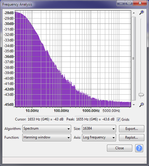
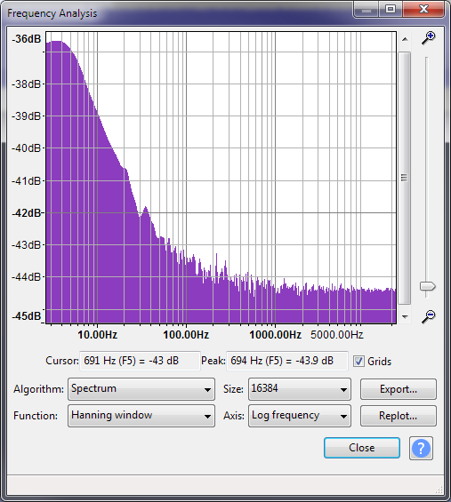
Use Audacity’s FFT feature to verify the noise file spectrums. Below are examples for the two -10 dBFS RMS files.
Pingback: Resistor johnson and flicker noise
Pingback: Resistor noise – the experiment and the results – Clockworks Signal Processing